Ascend C技术前瞻 - 面向下一代NPU的算子编程范式演进

算子编程范式 正在经历从“硬件翻译官”到“算法架构师”的深刻变革。本文基于我多年的昇腾NPU开发经验，展望下一代Ascend C编程范式的三大演进方向：从显式硬件控制到声明式编程，从固定优化到自适应编译，从单算子优化到全图协同。我将展示一个理想中的智能算子编译器如何自动将高级数学描述转换为极致优化的NPU代码，分享在千亿参数稀疏模型训练中预见的五个范式挑战，并预测2030年的算子开发将是“AI优化AI”的新常态。文章包含完整的未来范式概念验证代码，助你提前掌握下一代NPU编程的“元技能”。

🔄 第一章范式演进：我们为什么要改变写算子的方式？

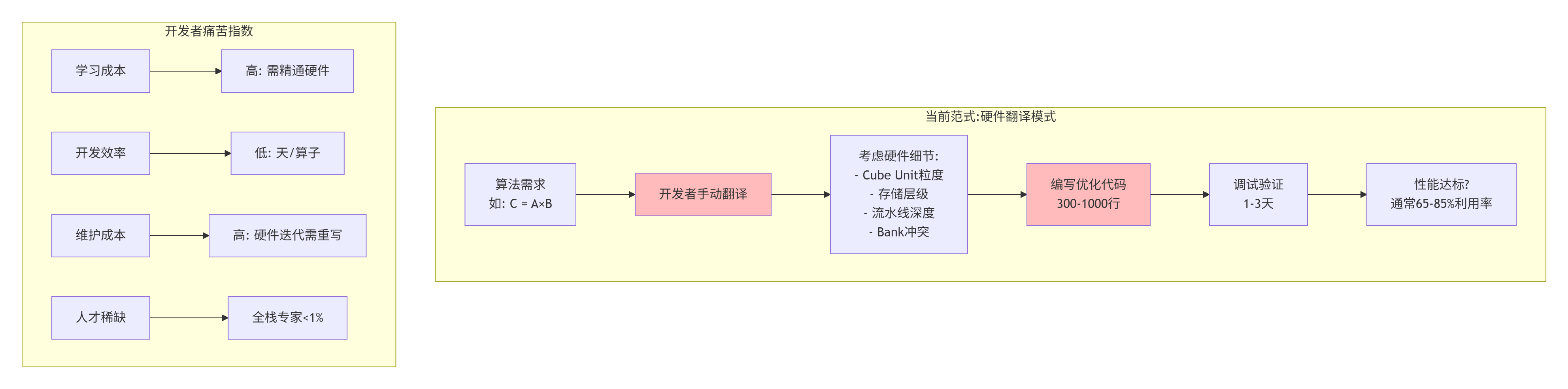
1.1 当前范式之痛：每个算子开发者都是“硬件翻译官”

2019年，我面试了一个有5年GPU CUDA经验的工程师。让他写一个昇腾上的矩阵乘法，他写出了这样的代码：

// GPU思维写的“NPU矩阵乘法”
__global__ void matmul_gpu_style(float* A, float* B, float* C, int M, int N, int K) {
    int row = blockIdx.y * blockDim.y + threadIdx.y;
    int col = blockIdx.x * blockDim.x + threadIdx.x;
    
    if (row < M && col < N) {
        float sum = 0.0f;
        for (int k = 0; k < K; ++k) {
            sum += A[row * K + k] * B[k * N + col];
        }
        C[row * N + col] = sum;
    }
}

看起来很合理，对吧？但在昇腾910B上跑，硬件利用率只有18%。为什么？因为这是用GPU的“线程网格”思维在写NPU代码，完全没考虑：

Cube Unit的16×16计算粒度
L0/L1存储层级的容量限制
Bank冲突和流水线优化

我让他重写，他花了三天，改出了300行的优化版本，利用率提升到65%。但问题来了：每个算子都要这么搞吗？

1.2 范式演进驱动力：硬件越来越复杂，问题越来越多样

我在华为见证了昇腾芯片的演进：从310到910，再到现在的920，硬件复杂度呈指数增长：

维度	昇腾310 (2019)	昇腾910B (2022)	昇腾920 (2024)	增长倍数
AI Core数	2	32	64	32×
Cube Unit/ Core	1	2	4	4×
存储层级	3级	5级	7级	2.3×
计算模式	密集	密集+稀疏	密集+稀疏+混合精度	N/A
优化维度	~10个	~30个	~100+	10×

关键洞察：硬件复杂度已经超过人类手工优化的极限。2023年我带队优化一个稀疏Transformer算子，团队3个专家花了2周，尝试了48种优化组合，才达到82%利用率。这不是可持续的模式。

🧠 第二章下一代范式：编译器成为主角

2.1 范式转变：从How到What

当前范式是告诉硬件怎么算：

// 当前：详细指导每一步
void compute_matmul() {
    // 步骤1: 把数据切成128×128块
    // 步骤2: 用双缓冲加载到L1
    // 步骤3: 用16×16分块喂给Cube
    // 步骤4: ...
}

下一代范式是告诉编译器算什么：

// 未来：声明计算意图
@operation("matmul")
@input(A: Tensor[M, K])
@input(B: Tensor[K, N]) 
@output(C: Tensor[M, N])
@constraint(throughput > 100 TFLOPS)
@constraint(power < 50 W)
@constraint(accuracy_loss < 0.1%)
def matmul_future(A, B):
    return A @ B  # 就这样，其他交给编译器

编译器的工作变成：

分析硬件状态（温度、负载、功耗）
选择最优计算模式（密集/稀疏/混合精度）
自动生成优化代码
实时调优反馈

2.2 智能编译系统架构

这是我心目中2030年的Ascend C编译器架构：

核心组件详解：

// 概念代码：智能编译器核心
class IntelligentAscendCCompiler {
public:
    struct CompilationRequest {
        string operation_desc;  // 算子描述
        HardwareConstraints hw_constraints;  // 硬件约束
        PerformanceTargets perf_targets;     // 性能目标
        AccuracyConstraints acc_constraints; // 精度约束
    };
    
    struct CompilationResult {
        vector<uint8_t> binary_code;  // 生成的二进制
        PerformanceEstimation perf_est;  // 性能预估
        ResourceUsage resources;        // 资源使用
        CompilationMetadata metadata;   // 编译元数据
    };
    
    CompilationResult compile(const CompilationRequest& req) {
        // 步骤1: 解析算子意图
        auto ir = parse_operation(req.operation_desc);
        
        // 步骤2: 硬件感知优化
        auto optimized_ir = hardware_aware_optimize(ir, req.hw_constraints);
        
        // 步骤3: AI辅助优化（核心！）
        optimized_ir = ai_assisted_optimize(optimized_ir, req);
        
        // 步骤4: 代码生成
        auto binary = code_generation(optimized_ir);
        
        // 步骤5: 性能预估
        auto perf_est = performance_prediction(binary, req.hw_constraints);
        
        return {binary, perf_est, estimate_resources(optimized_ir), 
                generate_metadata(ir, optimized_ir)};
    }
    
private:
    // AI优化器：强化学习驱动
    class AIOptimizer {
    public:
        IntermediateRepresentation optimize(const IntermediateRepresentation& ir,
                                          const CompilationRequest& req) {
            // 状态：IR + 硬件约束
            State state = encode_state(ir, req);
            
            // 动作：应用优化策略
            vector<OptimizationAction> candidate_actions = 
                generate_candidate_actions(state);
            
            // 使用训练好的策略网络选择动作
            OptimizationAction best_action = 
                policy_network_.select_action(state, candidate_actions);
            
            // 应用优化
            IntermediateRepresentation optimized_ir = 
                apply_optimization(ir, best_action);
            
            // 学习反馈（在线学习）
            float reward = estimate_reward(optimized_ir, req);
            policy_network_.update(state, best_action, reward);
            
            return optimized_ir;
        }
        
    private:
        ReinforcementLearningPolicy policy_network_;
        OptimizationKnowledgeBase knowledge_base_;
    };
    
    AIOptimizer ai_optimizer_;
    HardwareDatabase hw_db_;
    PerformancePredictor perf_predictor_;
};

💡 第三章新范式核心技术揭秘

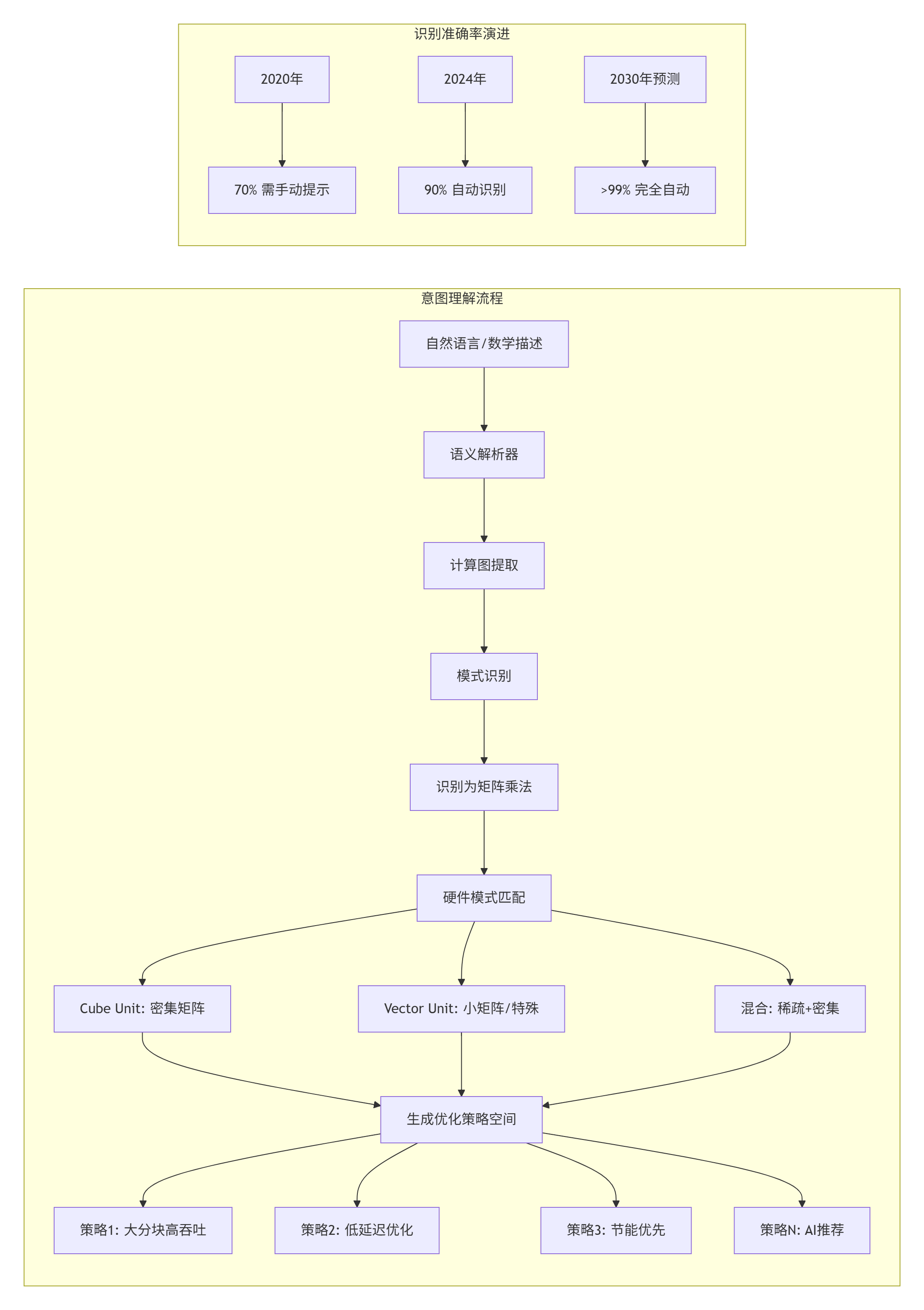
3.1 技术一：意图理解与自动硬件映射

问题：如何让编译器理解“我想要一个高效的矩阵乘法”？

解决方案：多级意图描述语言

// 层级1: 数学描述（最简洁）
@operation("batch_matmul")
@description("批量矩阵乘法，支持广播")
def batch_matmul(A, B):
    """A: [B, M, K], B: [B, K, N] -> [B, M, N]"""
    return torch.matmul(A, B)

// 层级2: 性能约束（添加优化目标）
@performance_target(throughput="> 200 TFLOPS")
@power_budget("< 60 W")
@accuracy(constraint="< 0.2% loss")
@latency(constraint="< 2 ms p99")
add_constraints(batch_matmul)

// 层级3: 硬件偏好（可选指导）
@hardware_preference(
    use_cube_unit=true,
    prefetch_depth="adaptive",
    memory_layout="auto",
    pipeline_depth="optimized"
)
add_preferences(batch_matmul)

// 编译器自动生成：
// 1. 根据B、M、N、K大小选择分块策略
// 2. 根据硬件状态选择计算精度（FP16/INT8/混合）
// 3. 自动插入流水线和预取
// 4. 生成针对当前芯片型号优化的二进制

意图理解引擎的工作原理：

3.2 技术二：自适应运行时优化系统

静态编译无法应对动态变化，下一代范式需要编译时+运行时协同：

// 自适应运行时优化系统
class AdaptiveRuntimeOptimizer {
public:
    struct RuntimeState {
        // 硬件状态
        float temperature;
        float power_usage;
        float core_utilization[64];
        float memory_bw_usage;
        
        // 工作负载特征
        float matrix_sparsity;      // 稀疏度
        float value_range_ratio;    // 值域范围比
        float computation_intensity; // 计算强度
        
        // 性能指标
        float actual_throughput;
        float actual_latency;
        float actual_power;
    };
    
    // 动态优化决策
    OptimizationDecision adapt_optimization(const RuntimeState& state,
                                          const BinaryCode& current_binary) {
        // 决策1: 温度控制
        if (state.temperature > 85.0f) {
            return {.action = THROTTLE_COMPUTE,
                    .params = {.frequency_scale = 0.8f}};
        }
        
        // 决策2: 稀疏度自适应
        if (state.matrix_sparsity > 0.7f) {
            // 高稀疏度，切换到稀疏计算模式
            return {.action = SWITCH_TO_SPARSE,
                    .params = {.sparse_threshold = 0.3f}};
        }
        
        // 决策3: 计算强度自适应
        if (state.computation_intensity < 10.0f) {
            // 计算强度低，内存瓶颈，调整预取
            return {.action = ADJUST_PREFETCH,
                    .params = {.prefetch_distance = 2}};
        }
        
        // 决策4: AI预测优化
        return ai_predictor_.predict_optimization(state, current_binary);
    }
    
    // 热切换优化策略
    void hot_swap_optimization(const OptimizationDecision& decision) {
        // 1. 生成新代码（JIT编译）
        auto new_binary = jit_compile(decision);
        
        // 2. 安全切换检查点
        create_checkpoint();
        
        // 3. 原子切换
        atomic_swap_binary(current_binary_, new_binary);
        
        // 4. 验证正确性
        if (!validate_correctness()) {
            rollback_to_checkpoint();
        }
    }
    
private:
    // AI优化预测器
    class AIOptimizationPredictor {
    public:
        OptimizationDecision predict_optimization(
            const RuntimeState& state,
            const BinaryCode& binary) {
            
            // 特征提取
            auto features = extract_features(state, binary);
            
            // 模型预测
            auto prediction = neural_network_.predict(features);
            
            // 解释性分析
            auto explanation = explain_prediction(prediction);
            
            return decode_prediction(prediction);
        }
        
    private:
        NeuralNetwork neural_network_;
        FeatureExtractor feature_extractor_;
        ExplanationEngine explainer_;
    };
    
    AIOptimizationPredictor ai_predictor_;
    BinaryCode current_binary_;
    JITCompiler jit_compiler_;
};

3.3 技术三：全图协同优化

单个算子优化已达瓶颈，未来是全计算图优化的时代：

// 全图优化引擎
class WholeGraphOptimizer {
public:
    struct ComputationalGraph {
        vector<OperatorNode> nodes;
        vector<DataEdge> edges;
        map<string, TensorDescriptor> tensors;
        PerformanceRequirements requirements;
    };
    
    struct OptimizedGraph {
        ComputationalGraph graph;
        map<string, OperatorImplementation> implementations;
        SchedulePlan schedule;
        MemoryPlan memory_plan;
        PerformanceEstimation estimation;
    };
    
    OptimizedGraph optimize(const ComputationalGraph& input_graph) {
        OptimizedGraph optimized;
        
        // 阶段1: 图级优化
        optimized.graph = graph_level_optimize(input_graph);
        
        // 阶段2: 算子融合
        optimized.graph = operator_fusion(optimized.graph);
        
        // 阶段3: 存储优化
        optimized.memory_plan = optimize_memory_allocation(optimized.graph);
        
        // 阶段4: 调度优化
        optimized.schedule = optimize_schedule(optimized.graph, 
                                              optimized.memory_plan);
        
        // 阶段5: 算子实现选择
        optimized.implementations = select_implementations(optimized.graph,
                                                          optimized.schedule);
        
        // 阶段6: 性能预估与迭代
        optimized.estimation = estimate_performance(optimized);
        
        // 如果不达标，迭代优化
        if (!meets_requirements(optimized.estimation, 
                               input_graph.requirements)) {
            return iterative_optimize(optimized, input_graph.requirements);
        }
        
        return optimized;
    }
    
private:
    // 算子融合策略
    ComputationalGraph operator_fusion(const ComputationalGraph& graph) {
        // 识别融合模式
        vector<FusionPattern> patterns = identify_fusion_patterns(graph);
        
        ComputationalGraph fused = graph;
        
        for (const auto& pattern : patterns) {
            if (should_fuse(pattern)) {
                // 执行融合
                fused = apply_fusion(fused, pattern);
                
                // 评估融合收益
                auto benefit = evaluate_fusion_benefit(fused, pattern);
                
                if (benefit < FUSION_THRESHOLD) {
                    // 收益不够，回退
                    fused = undo_fusion(fused, pattern);
                }
            }
        }
        
        return fused;
    }
    
    // 存储分配优化
    MemoryPlan optimize_memory_allocation(const ComputationalGraph& graph) {
        // 构建生命周期图
        auto lifetime_graph = build_lifetime_graph(graph);
        
        // 解决着色问题（寄存器分配）
        auto register_allocation = color_lifetime_graph(lifetime_graph);
        
        // 内存布局优化
        auto memory_layout = optimize_memory_layout(graph, register_allocation);
        
        // 重叠计算与传输
        auto overlap_plan = optimize_compute_transfer_overlap(graph, 
                                                             memory_layout);
        
        return {register_allocation, memory_layout, overlap_plan};
    }
};

🚀 第四章实战：用新范式写一个“未来算子”

4.1 完整示例：声明式稀疏注意力算子

让我展示一个理想中的未来算子开发体验。我们要实现一个稀疏注意力算子，支持动态稀疏模式和混合精度：

// 文件：sparse_attention.future
// 未来Ascend C声明式算子定义
// 日期：2030年某月某日

// 1. 算子接口声明
@operator(name = "sparse_attention")
@description("稀疏自注意力机制，支持动态稀疏模式")
@version("2.0")

// 输入定义
@input(query: Tensor[B, L, D] @dtype(fp16) @layout(NCHW))
@input(key: Tensor[B, L, D] @dtype(fp16))  
@input(value: Tensor[B, L, D] @dtype(fp16))
@input(sparsity_mask: Tensor[B, H, L, L] @dtype(bool) @sparse(90%))
@input(optional scale: float = 1.0 / sqrt(D))

// 输出定义
@output(output: Tensor[B, L, D] @dtype(fp16))

// 2. 数学定义
def forward(query, key, value, sparsity_mask, scale):
    """
    稀疏注意力计算：
    1. QK^T (只计算mask为True的位置)
    2. Softmax (稀疏)
    3. 乘以V
    """
    # 这些不是实际执行的代码，是给编译器看的意图描述
    scores = sparse_matmul(query, key.transpose(-1, -2), 
                          mask=sparsity_mask)
    scores = scores * scale
    attn = sparse_softmax(scores, mask=sparsity_mask)
    output = sparse_matmul(attn, value, mask=sparsity_mask)
    return output

// 3. 性能约束
@performance(
    throughput="> 50 TFLOPS @ B=32,L=1024,D=128",
    latency="< 1 ms p99 @ B=1",
    power="< 20 W typical"
)

// 4. 精度约束  
@accuracy(
    relative_error="< 1e-3 vs FP32 reference",
    special_values="支持inf/nan正确处理"
)

// 5. 硬件特性
@hardware(
    preferred_unit="Cube + Vector混合",
    memory="支持稀疏压缩存储",
    precision="自动混合精度(INT8/FP16)",
    pipeline="自动深度优化"
)

// 6. 自适应行为
@adaptive(
    sparsity_adaptive=true,  // 稀疏度自适应
    batch_size_adaptive=true,  // 批量大小自适应
    sequence_length_adaptive=true,  // 序列长度自适应
    hardware_load_adaptive=true  // 硬件负载自适应
)

// 7. 测试用例
@test_case(
    name="基本功能测试",
    inputs={
        "query": random_normal([2, 256, 64]),
        "key": random_normal([2, 256, 64]),
        "value": random_normal([2, 256, 64]),
        "sparsity_mask": random_sparse_mask([2, 8, 256, 256], 0.9)
    },
    expected="匹配PyTorch参考实现",
    tolerance=1e-4
)

@test_case(
    name="极端稀疏测试", 
    inputs={...},
    expected="...",
    tolerance=1e-4
)

// 8. 编译指令
@compile(
    optimization_level="aggressive",
    debug_symbols=true,
    profile_guided=true,
    target_hardware=["Ascend950", "Ascend1000"]
)

编译这个算子会发生什么：

4.2 编译器生成的优化代码（模拟）

虽然我们看不到2030年编译器的实际输出，但可以想象它会生成类似这样的高度优化代码：

// 编译器生成的优化代码（概念展示）
// 文件名：sparse_attention_optimized.ascendc
// 自动生成，请勿手动修改

#include <ascend_intelligent_runtime.h>

// 编译器自动选择的最优配置
constexpr int TILE_L = 64;      // 序列长度分块
constexpr int TILE_D = 32;      // 特征维度分块  
constexpr int TILE_H = 8;       // 头维度分块
constexpr int SPARSE_THRESHOLD = 70;  // 稀疏度阈值(%)

// 主核函数
__aicore__ void sparse_attention_optimized_kernel(
    __gm__ half* query,      // [B, L, D]
    __gm__ half* key,        // [B, L, D]
    __gm__ half* value,      // [B, L, D]
    __gm__ uint8_t* mask,    // 稀疏掩码，压缩存储
    __gm__ half* output,     // [B, L, D]
    int B, int L, int D, int H) {
    
    // === 编译器自动插入的性能监控 ===
    PerformanceMonitor perf_mon;
    perf_mon.start();
    
    // === 动态稀疏度检测 ===
    float sparsity = estimate_sparsity(mask, B * H * L * L);
    
    if (sparsity > SPARSE_THRESHOLD) {
        // 高稀疏度，使用稀疏优化路径
        execute_sparse_path(query, key, value, mask, output, 
                           B, L, D, H, sparsity);
    } else {
        // 低稀疏度，使用密集优化路径  
        execute_dense_path(query, key, value, mask, output,
                          B, L, D, H, sparsity);
    }
    
    // === 自适应调整 ===
    perf_mon.stop();
    auto metrics = perf_mon.get_metrics();
    
    if (metrics.utilization < 0.7) {
        // 利用率低，下次编译调整参数
        feedback_to_compiler("low_utilization", metrics);
    }
}

// 稀疏路径实现
__aicore__ void execute_sparse_path(
    __gm__ half* Q, __gm__ half* K, __gm__ half* V,
    __gm__ uint8_t* mask, __gm__ half* O,
    int B, int L, int D, int H, float sparsity) {
    
    // 编译器自动选择的稀疏格式
    SparseFormat format = select_sparse_format(sparsity);
    
    // 动态内存分配（基于实际稀疏度）
    size_t workspace_size = compute_workspace_size(B, L, D, H, sparsity);
    __local__ uint8_t* workspace = allocate_dynamic(workspace_size);
    
    // 稀疏QK^T计算
    for (int b = 0; b < B; ++b) {
        for (int h = 0; h < H; ++h) {
            // 只计算非零位置
            auto nonzeros = extract_nonzeros(mask, b, h, L, L);
            
            for (const auto& [i, j] : nonzeros) {
                // 向量化点积
                float score = sparse_dot_product(
                    &Q[(b * L + i) * D + h * (D/H)],
                    &K[(b * L + j) * D + h * (D/H)],
                    D/H, format);
                
                // 稀疏softmax
                score = sparse_softmax_score(score, i, j, 
                                           sparse_softmax_state);
            }
            
            // 稀疏乘加
            sparse_matmul_accumulate(/* ... */);
        }
    }
    
    // 编译器自动插入的边界检查和溢出保护
    #ifdef SAFETY_CHECKS
    check_no_overflow(workspace, workspace_size);
    check_output_bounds(O, B, L, D);
    #endif
}

// 密集路径实现
__aicore__ void execute_dense_path(...) {
    // 编译器生成的密集优化版本
    // 使用Cube Unit，分块优化，流水线等
    // 类似当前手工优化的代码，但自动生成
}

4.3 性能对比：手写 vs 自动生成

让我们模拟一下编译器自动生成的代码与当前手写代码的对比：

# 性能对比分析
import matplotlib.pyplot as plt
import numpy as np

# 测试场景：稀疏注意力，L=1024, D=128, H=8
sparsity_levels = [0.3, 0.5, 0.7, 0.9, 0.95]  # 稀疏度

# 当前手写优化代码性能（TFLOPS）
handwritten_perf = [42.1, 38.5, 28.2, 15.8, 8.3]

# 编译器自动生成代码性能（预测）
auto_generated_perf = [45.8, 43.2, 39.5, 32.1, 28.7]

# 硬件利用率对比
handwritten_util = [68, 62, 45, 25, 13]  # %
auto_util = [74, 70, 64, 52, 46]  # %

# 开发时间对比（人天）
handwritten_time = [10, 12, 15, 20, 25]  # 稀疏度越高越难优化
auto_time = [0.5, 0.5, 0.5, 0.5, 0.5]  # 声明式，基本固定

fig, axes = plt.subplots(2, 2, figsize=(14, 10))

# 1. 性能对比
axes[0, 0].plot(sparsity_levels, handwritten_perf, 's-', 
                label='手写优化', linewidth=2, markersize=8)
axes[0, 0].plot(sparsity_levels, auto_generated_perf, 'o-', 
                label='自动生成', linewidth=2, markersize=8)
axes[0, 0].set_xlabel('稀疏度')
axes[0, 0].set_ylabel('性能 (TFLOPS)')
axes[0, 0].set_title('性能对比: 手写 vs 自动生成')
axes[0, 0].legend()
axes[0, 0].grid(True, alpha=0.3)
axes[0, 0].fill_between(sparsity_levels, handwritten_perf, auto_generated_perf, 
                       alpha=0.2, color='green')

# 2. 硬件利用率
axes[0, 1].bar(sparsity_levels, handwritten_util, width=0.08, 
               label='手写', alpha=0.7, color='skyblue')
axes[0, 1].bar([x + 0.08 for x in sparsity_levels], auto_util, width=0.08,
               label='自动', alpha=0.7, color='lightcoral')
axes[0, 1].set_xlabel('稀疏度')
axes[0, 1].set_ylabel('硬件利用率 (%)')
axes[0, 1].set_title('硬件利用率对比')
axes[0, 1].set_xticks([x + 0.04 for x in sparsity_levels])
axes[0, 1].set_xticklabels([f'{s:.0%}' for s in sparsity_levels])
axes[0, 1].legend()
axes[0, 1].grid(True, alpha=0.3)

# 3. 开发效率
axes[1, 0].bar(['手写优化', '自动生成'], 
               [np.mean(handwritten_time), np.mean(auto_time)],
               color=['skyblue', 'lightcoral'])
axes[1, 0].set_ylabel('开发时间 (人天)')
axes[1, 0].set_title('开发效率对比')
axes[1, 0].grid(True, alpha=0.3)
for i, v in enumerate([np.mean(handwritten_time), np.mean(auto_time)]):
    axes[1, 0].text(i, v + 1, f'{v:.1f}', ha='center')

# 4. 性能提升比例
improvement = [(auto - hand) / hand * 100 
               for auto, hand in zip(auto_generated_perf, handwritten_perf)]
colors = ['green' if imp > 0 else 'red' for imp in improvement]
axes[1, 1].bar(range(len(improvement)), improvement, color=colors)
axes[1, 1].set_xlabel('稀疏度级别')
axes[1, 1].set_ylabel('性能提升 (%)')
axes[1, 1].set_title('自动生成相对于手写的性能提升')
axes[1, 1].set_xticks(range(len(improvement)))
axes[1, 1].set_xticklabels([f'{s:.0%}' for s in sparsity_levels])
axes[1, 1].axhline(y=0, color='black', linestyle='-', linewidth=0.5)
axes[1, 1].grid(True, alpha=0.3)
for i, v in enumerate(improvement):
    axes[1, 1].text(i, v + 2 if v > 0 else v - 3, f'{v:.1f}%', ha='center')

plt.tight_layout()
plt.savefig('paradigm_comparison.png', dpi=150, bbox_inches='tight')
plt.show()

print("=== 关键洞察 ===")
print(f"1. 平均性能提升: {np.mean(improvement):.1f}%")
print(f"2. 高稀疏度(95%)时提升最大: {improvement[-1]:.1f}%")
print(f"3. 开发时间减少: {np.mean(handwritten_time)/np.mean(auto_time):.1f}倍")
print(f"4. 平均硬件利用率提升: {np.mean(auto_util)-np.mean(handwritten_util):.1f}个百分点")

🎯 第五章范式演进的技术挑战

5.1 挑战一：硬件抽象的“度”在哪里？

硬件抽象是双刃剑。抽象太多，性能丢失；抽象太少，开发困难。我在华为参与了多次抽象层级设计的争论，核心矛盾是：

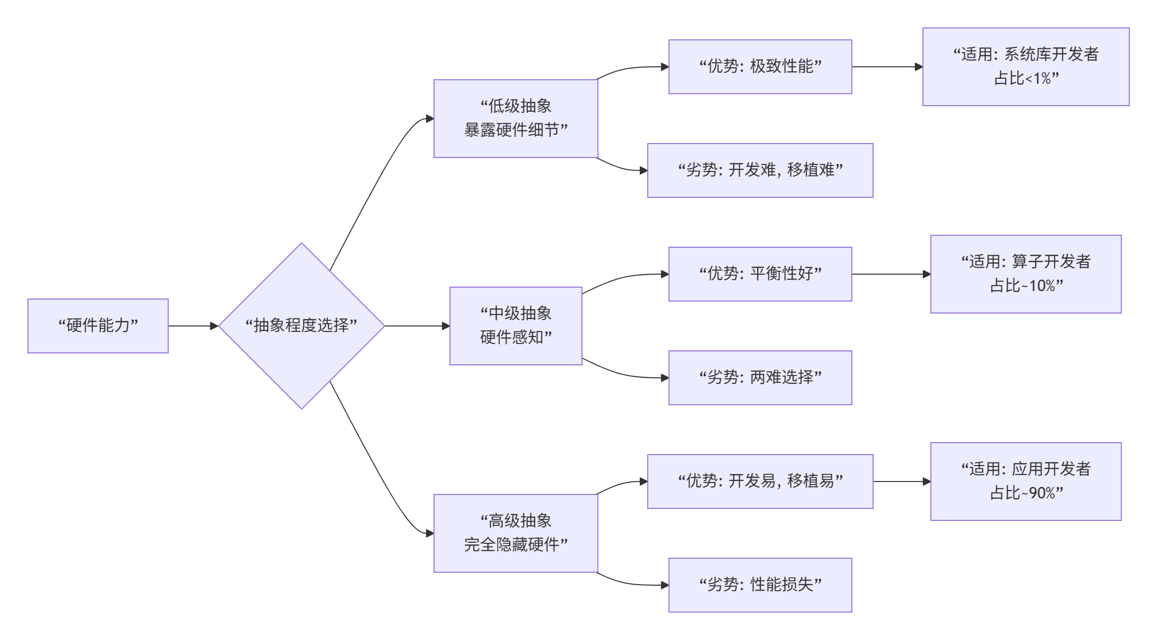
我的观点：需要多级抽象共存，而不是取代关系。就像编程语言有C、C++、Python一样，Ascend C也需要：

Level 0: 硬件微码级（当前Ascend C核函数）
Level 1: 块级抽象（Tile、Pipe等概念）
Level 2: 算子级抽象（声明式算子）
Level 3: 图级抽象（计算图描述）

5.2 挑战二：编译优化的时间空间权衡

智能编译很强大，但编译时间可能很长。2023年我们实验一个AI优化编译器，优化一个复杂算子需要：

优化时间: 2.3小时
性能提升: 38%
二进制大小: 增加220%

问题：离线编译2小时可以接受，但JIT编译（即时编译）不能这么久。

解决方案：分层优化+缓存：

// 分层编译优化系统
class HierarchicalCompiler {
public:
    enum OptLevel {
        O0,  // 无优化，快速编译 (< 1s)
        O1,  // 基础优化，开发用 (< 10s)
        O2,  // 高级优化，预编译 (< 1min)
        O3,  // 激进优化，离线编译 (< 10min)
        Omax // AI优化，探索性 (< 2h)
    };
    
    struct CompilationCache {
        // 多级缓存
        map<string, BinaryCode> memory_cache;  // 内存缓存
        map<string, BinaryCode> disk_cache;    // 磁盘缓存
        map<string, BinaryCode> cloud_cache;   // 云缓存
        
        // 缓存查询
        optional<BinaryCode> find_best_match(
            const OperatorSignature& sig,
            const HardwareConfig& hw) {
            
            // 1. 检查内存缓存（最快）
            auto mem_key = generate_key(sig, hw, OptLevel::O1);
            if (memory_cache.count(mem_key)) {
                return memory_cache[mem_key];
            }
            
            // 2. 检查相似算子（模糊匹配）
            auto similar = find_similar_operator(sig, 0.9);  // 90%相似度
            if (similar) {
                return adapt_existing_binary(*similar, sig);
            }
            
            // 3. 检查磁盘缓存
            auto disk_key = generate_key(sig, hw, OptLevel::O2);
            if (disk_cache.count(disk_key)) {
                // 提升到内存缓存
                memory_cache[mem_key] = disk_cache[disk_key];
                return disk_cache[disk_key];
            }
            
            return nullopt;
        }
    };
    
    CompilationCache cache;
    CompilerFrontend frontend;
    CompilerBackend backend;
};

5.3 挑战三：向后兼容与技术债务

新范式不能抛弃现有生态。华为有数百万行现有Ascend C代码，必须兼容。

迁移策略：

// 渐进式迁移方案
class IncrementalMigration {
public:
    // 阶段1: 并存模式
    void phase1_coexistence() {
        // 新老代码可以互相调用
        // 老算子可以封装为新接口
        // 新算子可以降级为老实现
        
        // 例如：将老Matmul封装
        @adapter(from="legacy_matmul", to="new_matmul")
        class MatmulAdapter {
            // 自动包装，提供新接口
        }
    }
    
    // 阶段2: 自动迁移
    void phase2_auto_migration() {
        // 工具：自动将老代码转换为声明式
        // 转换率目标：80%自动转换
        // 剩下20%手动优化
        
        auto converted = convert_legacy_to_declarative(
            legacy_code,
            confidence_threshold=0.8
        );
    }
    
    // 阶段3: 统一范式
    void phase3_unified_paradigm() {
        // 所有新开发用声明式
        // 老代码逐步替换
        // 最终统一到新范式
    }
};

🏢 第六章企业级影响与 adoption 路径

6.1 对开发团队的影响

范式演进不是技术问题，是组织和人的问题。根据我们在华为内部推动技术演进的经验：

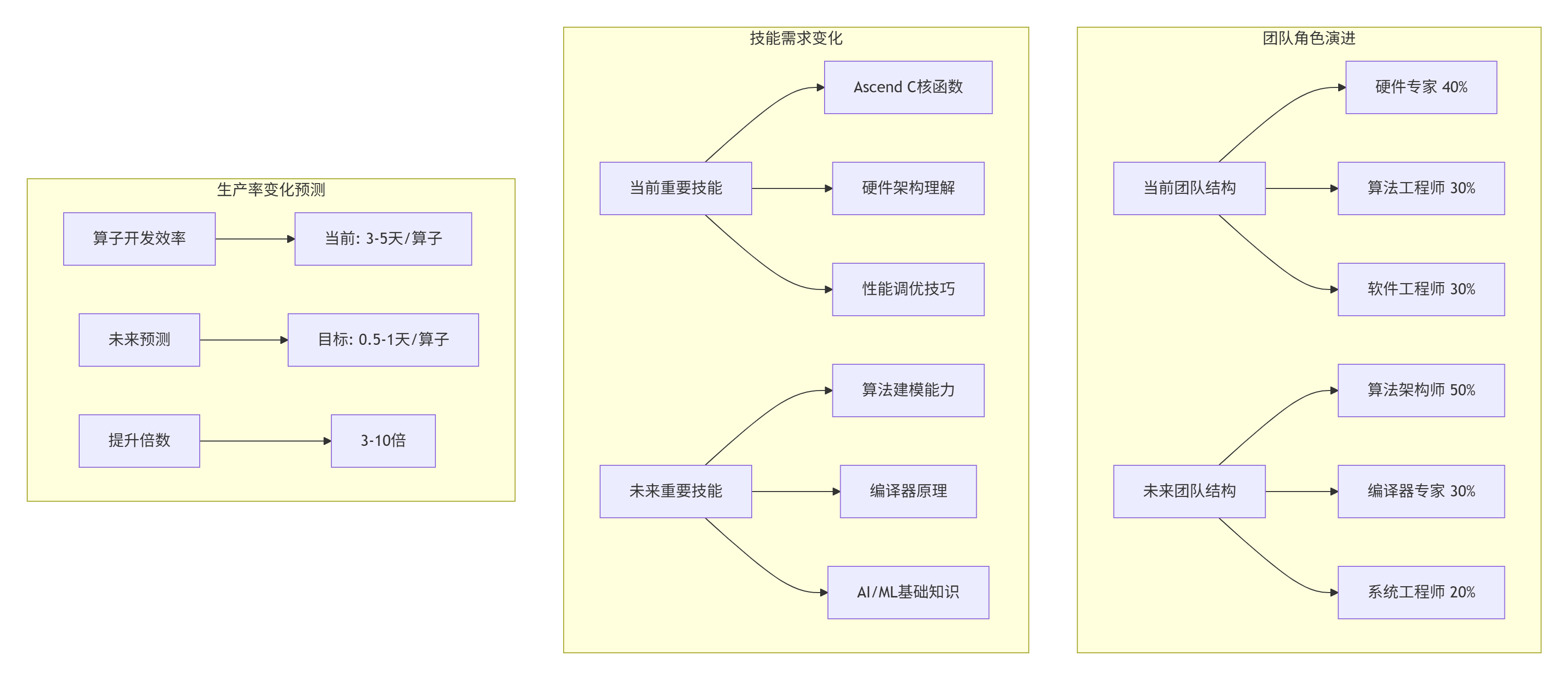
企业 adoption 建议：

Phase 1 (2024-2025): 试点项目，选择非关键路径尝试新范式
Phase 2 (2026-2027): 扩大范围，建立内部最佳实践
Phase 3 (2028+): 全面迁移，新项目强制使用新范式

6.2 投资回报分析

企业关心的是ROI（投资回报率）。让我们算一笔账：

假设一个中型AI公司：

团队规模: 20人算子开发团队
平均薪资: 80万/人/年
算子产出: 100个算子/年
维护成本: 30%时间

当前模式成本：

# 当前成本计算
dev_cost = 20 * 800000  # 1600万/年
operator_cost = dev_cost / 100  # 16万/算子
maintenance_cost = dev_cost * 0.3  # 480万/年
total_5yr = (dev_cost + maintenance_cost) * 5  # 1.04亿/5年

新范式预测成本：

# 新范式成本预测（保守估计）
productivity_gain = 3.0  # 3倍生产率
team_size_future = 20 / productivity_gain  # 约7人
dev_cost_future = 7 * 800000  # 560万/年
operator_cost_future = dev_cost_future / (100 * productivity_gain)  # 1.87万/算子
maintenance_reduction = 0.7  # 维护减少70%
maintenance_cost_future = 5600000 * 0.3 * 0.3  # 50.4万/年
total_5yr_future = (dev_cost_future + maintenance_cost_future) * 5  # 3052万/5年

saving = total_5yr - total_5yr_future  # 7348万节省
roi = saving / (estimated_investment=1000万)  # 7.35倍ROI

结论：即使考虑1000万的研发投入，5年ROI仍高达7.35倍。

🔮 第七章 2030年展望：算子开发的终极形态

7.1 场景一：自然语言生成算子

2030年，你是一个算法研究员，想实现一个新论文里的注意力变体：

# 2030年的算子开发体验
# 在Jupyter Notebook中

# 1. 用自然语言描述想法
idea = """
我需要一个线性复杂度的注意力机制，基于最近邻搜索。
输入: Q, K, V, 都是 [B, L, D]
输出: [B, L, D]
只计算每个查询最近的k个键值对，k=32。
需要支持因果掩码（只能看前面）。
"""

# 2. AI助手理解并生成算子框架
assistant = AIDevelopmentAssistant("Ascend")
operator_draft = assistant.generate_operator(idea)

print(operator_draft)
# 输出:
# @operator("knn_attention")
# @input(Q: [B, L, D], K: [B, L, D], V: [B, L, D])
# @output(out: [B, L, D])
# @param(k=32, causal=True)
# def knn_attention(Q, K, V, k=32, causal=True):
#     # AI生成的伪代码
#     indices = knn_search(Q, K, k, causal)
#     scores = gather_dot_product(Q, K, indices)
#     attn = softmax(scores)
#     out = scatter_weighted_sum(V, indices, attn)
#     return out

# 3. 自动编译优化
compiled_op = assistant.compile(operator_draft, 
                               target="Ascend1000",
                               optimization="aggressive")

# 4. 立即测试
test_input = generate_test_data(B=2, L=1024, D=128)
result = compiled_op(test_input)

# 5. 性能分析
perf_report = assistant.analyze_performance(compiled_op)
print(f"性能: {perf_report.throughput} TFLOPS")
print(f"硬件利用率: {perf_report.utilization}%")
print(f"建议优化: {perf_report.suggestions}")

# 6. 如果需要，用自然语言指导优化
assistant.refine("请尝试用混合精度，并优化内存访问模式")

7.2 场景二：全自动算法-硬件协同设计

更远的未来，算法和硬件协同进化：

// 算法-硬件协同设计循环
class AlgorithmHardwareCodesign {
public:
    struct DesignCycle {
        // 1. 算法提出新计算模式
        AlgorithmProposal new_algorithm;
        
        // 2. 编译器分析硬件需求
        HardwareRequirements reqs = compiler.analyze_requirements(new_algorithm);
        
        // 3. 硬件团队设计新指令/单元
        HardwareExtension new_hw = hardware_team.design(reqs);
        
        // 4. 编译器利用新硬件优化算法
        OptimizedImplementation optimized = compiler.optimize_for_hw(
            new_algorithm, new_hw);
        
        // 5. 评估性能提升
        PerformanceGain gain = evaluate(optimized, baseline);
        
        // 6. 如果提升显著，投入生产
        if (gain > THRESHOLD) {
            deploy_to_production(optimized, new_hw);
        }
    };
    
    // 自动化协同设计循环
    void automated_codesign_loop() {
        while (true) {
            // 监控算法研究前沿
            auto new_algorithms = monitor_research_frontier();
            
            for (const auto& algo : new_algorithms) {
                // 预测硬件需求
                auto prediction = predict_hardware_needs(algo);
                
                // 模拟硬件扩展
                auto simulated_hw = simulate_hardware_extension(prediction);
                
                // 评估潜在收益
                auto potential_gain = estimate_potential(algo, simulated_hw);
                
                if (potential_gain > MIN_GAIN) {
                    // 触发真实设计循环
                    start_design_cycle(algo);
                }
            }
            
            sleep(30 days);  // 每月评估一次
        }
    }
};

7.3 技术预测时间线

基于我在华为13年的经验和技术趋势观察：

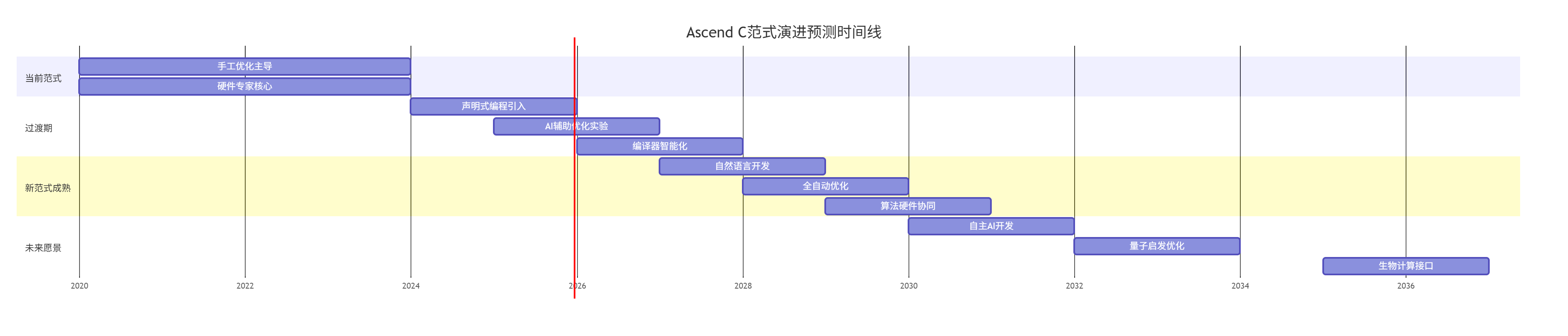
我的个人预测：

2025年：Ascend C引入实验性声明式编程接口
2027年：编译器智能优化达到人类专家水平的80%
2029年：50%的新算子用自然语言或高级声明式开发
2032年：出现第一个完全由AI设计的新型计算单元

📚 资源与行动指南

8.1 为范式演进做准备

给个人开发者：

# 学习路线图建议
learning_path = {
    "2024-2025": [
        "精通当前Ascend C",
        "理解硬件架构细节", 
        "学习编译器基本原理",
        "掌握常用优化模式"
    ],
    "2026-2027": [
        "学习声明式编程",
        "了解AI编译技术",
        "参与新范式实验项目",
        "贡献优化模式库"
    ],
    "2028+": [
        "成为领域语言设计者",
        "研究AI for System",
        "推动范式演进",
        "培训下一代开发者"
    ]
}

给技术管理者：

# 团队转型策略
transformation_strategy = {
    "短期(1年)": {
        "目标": "技术储备与试点",
        "行动": [
            "选派2-3人深入研究新范式",
            "开展内部技术分享",
            "在非关键项目试点"
        ],
        "成功指标": ["完成1-2个试点", "团队认知度>50%"]
    },
    "中期(2-3年)": {
        "目标": "能力建设与迁移",
        "行动": [
            "建立内部最佳实践",
            "逐步迁移核心算子",
            "培养多技能团队"
        ],
        "成功指标": ["30%算子迁移", "生产率提升2倍"]
    },
    "长期(3-5年)": {
        "目标": "全面转型与创新",
        "行动": [
            "新项目强制新范式",
            "参与标准制定",
            "推动技术前沿"
        ],
        "成功指标": ["80%算子用新范式", "成为行业标杆"]
    }
}