
基于 Ascend C 的 AsNumpy 性能调优指南
目录
摘要
本文对AsNumpy性能调优进行了系统总结。从性能分析方法论到分层优化策略,涵盖算法级优化、内存访问优化、计算图融合、混合精度、异步执行等关键技术。通过实际案例展示如何从初始实现到极致优化,实现从1x到112x的性能提升。提供完整工具链和实战代码,助你掌握NPU性能调优的完整方法论。
🚀 核心观点:性能调优不是一次性的魔法,而是系统性的工程科学。理解硬件特性,量化分析瓶颈,针对性优化,持续迭代验证。
1. 性能调优方法论
1.1 四步性能调优法

1.2 性能分析工具箱
# performance_analyzer.py
import asnp
import numpy as np
import time
from dataclasses import dataclass
from typing import Dict, List, Tuple
import matplotlib.pyplot as plt

@dataclass
class PerformanceMetrics:
    """性能指标"""
    execution_time_ms: float
    gflops: float
    memory_bandwidth_gbps: float
    compute_utilization: float
    memory_utilization: float
    operational_intensity: float
    roofline_distance: float
    bottleneck_type: str

class PerformanceAnalyzer:
    """性能分析器"""

    def analyze_roofline(self, operation, *args, compute_cost=None, memory_cost=None):
        """屋顶线分析"""
        # 测量性能
        exec_time = self.measure_execution_time(operation, *args)

        # 计算性能指标
        if compute_cost is None:
            compute_cost = self.estimate_compute_cost(operation, *args)
        if memory_cost is None:
            memory_cost = self.estimate_memory_cost(operation, *args)

        # 硬件规格
        peak_gflops = 393216.0  # Ascend 910B TFLOPS
        peak_bandwidth = 1200.0  # GB/s

        # 计算指标
        gflops = compute_cost / (exec_time * 1e9)
        bandwidth = memory_cost / (exec_time * 1e9)
        compute_util = gflops / peak_gflops
        memory_util = bandwidth / peak_bandwidth
        operational_intensity = compute_cost / memory_cost
        roofline_distance = gflops / min(peak_gflops, operational_intensity * peak_bandwidth)

        # 识别瓶颈
        bottleneck = self.identify_bottleneck(compute_util, memory_util, roofline_distance)

        return PerformanceMetrics(
            execution_time_ms=exec_time*1000,
            gflops=gflops,
            memory_bandwidth_gbps=bandwidth,
            compute_utilization=compute_util,
            memory_utilization=memory_util,
            operational_intensity=operational_intensity,
            roofline_distance=roofline_distance,
            bottleneck_type=bottleneck
        )

    def measure_execution_time(self, operation, *args, warmup=5, iterations=10):
        """精确测量执行时间"""
        # 预热
        for _ in range(warmup):
            result = operation(*args)
            if hasattr(result, 'asnumpy'):
                result.asnumpy()  # 确保计算完成

        # 测量
        times = []
        for _ in range(iterations):
            start = time.perf_counter()
            result = operation(*args)
            if hasattr(result, 'asnumpy'):
                result.asnumpy()  # 同步
            end = time.perf_counter()
            times.append(end - start)

        # 移除异常值
        times_sorted = sorted(times)
        trimmed_times = times_sorted[1:-1]  # 去除最大最小值
        return np.mean(trimmed_times)

    def identify_bottleneck(self, compute_util, memory_util, roofline_distance):
        """识别性能瓶颈"""
        if roofline_distance < 0.3:
            return "远离屋顶线"
        elif compute_util < 0.5 and memory_util > 0.7:
            return "计算绑定"
        elif compute_util > 0.7 and memory_util < 0.5:
            return "内存绑定"
        elif compute_util < 0.3 and memory_util < 0.3:
            return "启动/同步开销"
        elif 0.7 <= roofline_distance <= 1.0:
            return "接近峰值"
        else:
            return "平衡"

    def visualize_roofline(self, operations_metrics, save_path="roofline_analysis.png"):
        """可视化屋顶线分析"""
        fig, axes = plt.subplots(1, 2, figsize=(12, 5))

        # 屋顶线图
        peak_gflops = 393216
        peak_bandwidth = 1200

        oi = np.logspace(-2, 3, 100)
        roofline = np.minimum(peak_gflops, oi * peak_bandwidth)

        axes[0].loglog(oi, roofline, 'k-', linewidth=2, label='屋顶线')

        colors = plt.cm.tab10(np.linspace(0, 1, len(operations_metrics)))
        for idx, (op_name, metrics) in enumerate(operations_metrics.items()):
            axes[0].scatter(metrics.operational_intensity, metrics.gflops,
                           s=200, c=[colors[idx]], label=op_name, alpha=0.7)
            # 理论性能
            theoretical_gflops = min(peak_gflops,
                                     metrics.operational_intensity * peak_bandwidth)
            axes[0].plot([metrics.operational_intensity, metrics.operational_intensity],
                        [metrics.gflops, theoretical_gflops],
                        '--', color=colors[idx], alpha=0.5)

        axes[0].set_xlabel('运算强度 (FLOPs/Byte)')
        axes[0].set_ylabel('性能 (GFLOPS)')
        axes[0].set_title('屋顶线分析')
        axes[0].legend()
        axes[0].grid(True, alpha=0.3)

        # 瓶颈分析饼图
        bottleneck_counts = {
            '计算绑定': 0, '内存绑定': 0,
            '远离屋顶线': 0, '启动/同步': 0,
            '接近峰值': 0, '平衡': 0
        }

        for metrics in operations_metrics.values():
            bottleneck_counts[metrics.bottleneck_type] += 1

        wedges, texts, autotexts = axes[1].pie(
            bottleneck_counts.values(),
            labels=bottleneck_counts.keys(),
            autopct='%1.1f%%',
            colors=plt.cm.Set3(np.arange(len(bottleneck_counts)))
        )
        axes[1].set_title('性能瓶颈分布')

        plt.tight_layout()
        plt.savefig(save_path, dpi=300, bbox_inches='tight')
        plt.show()
2. 算法级优化
2.1 分块矩阵乘法
// tiled_matmul.cce
template<int BLOCK_M, int BLOCK_N, int BLOCK_K>
class TiledMatmulKernel {
public:
    __aicore__ inline void Process() {
        // 初始化输出
        for (int mi = 0; mi < BLOCK_M; ++mi) {
            for (int nj = 0; nj < BLOCK_N; ++nj) {
                output_[mi * BLOCK_N + nj] = 0.0f;
            }
        }

        // 分块计算
        for (int bk = 0; bk < k_; bk += BLOCK_K) {
            int k_start = bk;
            int k_end = min(bk + BLOCK_K, k_);

            // 加载A块
            LoadTileA(bk);

            // 加载B块
            LoadTileB(bk);

            // 块矩阵乘法
            for (int mi = 0; mi < BLOCK_M; ++mi) {
                for (int nj = 0; nj < BLOCK_N; ++nj) {
                    float sum = output_[mi * BLOCK_N + nj];

                    for (int ki = 0; ki < k_end - k_start; ++ki) {
                        float a_val = a_buffer_[mi * BLOCK_K + ki];
                        float b_val = b_buffer_[ki * BLOCK_N + nj];
                        sum += a_val * b_val;
                    }

                    output_[mi * BLOCK_N + nj] = sum;
                }
            }
        }
    }

private:
    __aicore__ inline void LoadTileA(int block_k) {
        // 合并内存访问
        for (int mi = 0; mi < BLOCK_M; ++mi) {
            int global_m = block_m_ * BLOCK_M + mi;
            if (global_m >= m_) break;

            for (int ki = 0; ki < BLOCK_K; ++ki) {
                int global_k = block_k + ki;
                float val = 0.0f;

                if (global_m < m_ && global_k < k_) {
                    val = a_global_[(global_m * k_) + global_k];
                }

                a_buffer_[mi * BLOCK_K + ki] = val;
            }
        }
    }
};分块大小优化策略:
def optimize_tile_sizes(m, n, k):
    """优化分块大小"""
    # 缓存大小
    L1_size = 32 * 1024  # 32KB
    L2_size = 512 * 1024  # 512KB
    register_size = 256  # 256个寄存器

    # 计算最优分块
    tile_sizes = []

    for tile_m in [16, 32, 64, 128, 256]:
        for tile_n in [16, 32, 64, 128, 256]:
            for tile_k in [16, 32, 64, 128, 256]:
                # 计算内存使用
                memory_usage = (tile_m * tile_k + tile_k * tile_n +
                               tile_m * tile_n) * 4  # bytes

                # 检查是否适合缓存
                if memory_usage < L1_size * 0.8:  # 80% 缓存利用率
                    # 计算寄存器使用
                    registers_needed = tile_m * tile_n
                    if registers_needed < register_size * 0.7:  # 70% 寄存器利用率
                        tile_sizes.append({
                            'M': tile_m,
                            'N': tile_n,
                            'K': tile_k,
                            'memory_usage': memory_usage,
                            'registers': registers_needed
                        })

    # 按内存使用排序
    tile_sizes.sort(key=lambda x: x['memory_usage'])

    return tile_sizes
2.2 计算图优化
# graph_optimizer.py
import networkx as nx
from typing import List, Dict, Tuple

class GraphOptimizer:
    """计算图优化器"""

    def fuse_operations(self, graph: nx.DiGraph, pattern: List[str]) -> nx.DiGraph:
        """算子融合优化"""
        optimized = graph.copy()
        fused_nodes = set()

        # 查找可融合的模式
        for i, node_id in enumerate(list(optimized.nodes())):
            if node_id in fused_nodes:
                continue

            node_data = optimized.nodes[node_id]
            if node_data.get('op_type') == pattern[0]:
                # 尝试匹配模式
                match = self._find_pattern(optimized, node_id, pattern)
                if match and len(match) == len(pattern):
                    # 执行融合
                    fused_node = self._create_fused_node(optimized, match, pattern)
                    optimized.add_node(fused_node['id'], **fused_node)

                    # 重新连接
                    for input_id in fused_node['inputs']:
                        optimized.add_edge(input_id, fused_node['id'])
                    for output_id in fused_node['outputs']:
                        optimized.add_edge(fused_node['id'], output_id)

                    # 标记已融合节点
                    fused_nodes.update(match)
                    optimized.remove_nodes_from(match)

        return optimized

    def _find_pattern(self, graph, start_node, pattern):
        """查找匹配模式"""
        if len(pattern) == 0:
            return []

        match = [start_node]
        current_node = start_node
        current_op = pattern[0]

        for i in range(1, len(pattern)):
            # 查找下一个节点
            successors = list(graph.successors(current_node))
            if len(successors) != 1:
                return None

            next_node = successors[0]
            if graph.nodes[next_node].get('op_type') != pattern[i]:
                return None

            match.append(next_node)
            current_node = next_node

        return match

    def schedule_operations(self, graph: nx.DiGraph) -> List[int]:
        """操作调度优化"""
        # 关键路径分析
        critical_path = self._find_critical_path(graph)

        # 计算优先级
        priorities = self._compute_priorities(graph, critical_path)

        # 资源约束调度
        schedule = self._resource_constrained_schedule(graph, priorities)

        return schedule

    def _find_critical_path(self, graph: nx.DiGraph) -> List[int]:
        """查找关键路径"""
        # 计算最长路径
        longest_paths = {}
        for node in graph.nodes():
            longest_paths[node] = 0

        # 拓扑排序
        topo_order = list(nx.topological_sort(graph))

        for node in topo_order:
            for successor in graph.successors(node):
                new_length = longest_paths[node] + graph.nodes[node].get('compute_cost', 1)
                if new_length > longest_paths[successor]:
                    longest_paths[successor] = new_length

        # 重建关键路径
        end_node = max(longest_paths, key=longest_paths.get)
        path = [end_node]

        while len(list(graph.predecessors(path[-1]))) > 0:
            predecessors = list(graph.predecessors(path[-1]))
            best_pred = max(predecessors, key=lambda x: longest_paths[x])
            path.append(best_pred)

        return list(reversed(path))

    def _compute_priorities(self, graph: nx.DiGraph, critical_path: List[int]) -> Dict[int, int]:
        """计算节点优先级"""
        priorities = {}
        cp_set = set(critical_path)

        for node in graph.nodes():
            if node in cp_set:
                # 关键路径节点优先级高
                priorities[node] = 100 + len(list(nx.descendants(graph, node)))
            else:
                # 非关键路径节点优先级低
                priorities[node] = len(list(nx.descendants(graph, node)))

        return priorities
3. 内存优化
3.1 内存访问优化
// memory_optimization.cce
class MemoryOptimizer {
public:
    // 优化内存访问模式
    __aicore__ inline void optimized_memory_access(float* data, int size) {
        // 合并访问优化
        for (int i = 0; i < size; i += 8) {
            // 加载8个连续元素
            float8 vec = load_vector8(data + i);

            // SIMD计算
            vec = vector_operation(vec);

            // 存储结果
            store_vector8(data + i, vec);
        }
    }

    // 共享内存优化
    __aicore__ inline void shared_memory_optimization(float* input,
                                                      float* output,
                                                      int M, int N, int K) {
        __shared__ float shared_mem[1024];  // 共享内存

        int tid = get_thread_idx();
        int num_threads = get_num_threads();

        // 合并全局内存访问
        for (int i = tid; i < M * K; i += num_threads) {
            shared_mem[tid] = input[i];
        }

        __syncthreads();  // 同步所有线程

        // 在共享内存中计算
        float sum = 0.0f;
        for (int i = 0; i < 1024; ++i) {
            sum += shared_mem[i];
        }

        // 合并全局内存写回
        for (int i = tid; i < M * N; i += num_threads) {
            output[i] = sum;
        }
    }

    // 向量化访问
    __aicore__ inline void vectorized_access(float* src, float* dst, int size) {
        // 向量化加载/存储
        for (int i = 0; i < size; i += 8) {
            // 加载8个浮点数
            float8 vec = load_vector8(src + i);

            // 向量化计算
            vec = vector_operation(vec);

            // 存储结果
            store_vector8(dst + i, vec);
        }
    }

    // 循环展开
    __aicore__ inline void loop_unrolling(float* a, float* b, float* c, int n) {
        const int UNROLL_FACTOR = 4;
        int i = 0;

        // 展开循环
        for (; i <= n - UNROLL_FACTOR; i += UNROLL_FACTOR) {
            float4 a_vec = load_vector4(a + i);
            float4 b_vec = load_vector4(b + i);
            float4 c_vec = a_vec + b_vec;
            store_vector4(c + i, c_vec);
        }

        // 处理剩余元素
        for (; i < n; ++i) {
            c[i] = a[i] + b[i];
        }
    }

    // 缓存友好访问
    __aicore__ inline void cache_friendly_access(float* matrix, int rows, int cols) {
        // 行主序访问
        for (int i = 0; i < rows; ++i) {
            for (int j = 0; j < cols; ++j) {
                matrix[i * cols + j] *= 2.0f;
            }
        }

        // 分块访问
        const int BLOCK_SIZE = 16;
        for (int i0 = 0; i0 < rows; i0 += BLOCK_SIZE) {
            for (int j0 = 0; j0 < cols; j0 += BLOCK_SIZE) {
                int i_end = min(i0 + BLOCK_SIZE, rows);
                int j_end = min(j0 + BLOCK_SIZE, cols);

                for (int i = i0; i < i_end; ++i) {
                    for (int j = j0; j < j_end; ++j) {
                        matrix[i * cols + j] += 1.0f;
                    }
                }
            }
        }
    }

private:
    __aicore__ inline float8 load_vector8(const float* ptr) {
        // 向量化加载
        float8 vec;
        #pragma unroll
        for (int i = 0; i < 8; ++i) {
            vec[i] = ptr[i];
        }
        return vec;
    }

    __aicore__ inline void store_vector8(float* ptr, float8 vec) {
        // 向量化存储
        #pragma unroll
        for (int i = 0; i < 8; ++i) {
            ptr[i] = vec[i];
        }
    }

    __aicore__ inline float8 vector_operation(float8 vec) {
        // 向量化操作
        float8 result;
        #pragma unroll
        for (int i = 0; i < 8; ++i) {
            result[i] = vec[i] * 2.0f + 1.0f;
        }
        return result;
    }
};
3.2 内存层次优化策略
# memory_hierarchy_optimizer.py
def optimize_memory_hierarchy(data_shape, compute_type="matmul"):
    """内存层次优化"""
    # 硬件特性
    hw_specs = {
        'register_size': 256,  # 寄存器数
        'shared_mem_size': 96 * 1024,  # 共享内存
        'L1_cache_size': 32 * 1024,  # L1缓存
        'L2_cache_size': 512 * 1024,  # L2缓存
        'global_mem_bandwidth': 1200e9,  # 全局内存带宽
    }

    # 分析数据访问模式
    if compute_type == "matmul":
        # 矩阵乘法优化
        tile_config = optimize_matmul_tiling(data_shape, hw_specs)

    elif compute_type == "convolution":
        # 卷积优化
        tile_config = optimize_conv_tiling(data_shape, hw_specs)

    elif compute_type == "reduction":
        # 归约优化
        tile_config = optimize_reduction_tiling(data_shape, hw_specs)

    return tile_config

def optimize_matmul_tiling(shape, hw_specs):
    """矩阵乘法分块优化"""
    M, N, K = shape

    best_config = None
    best_score = -float('inf')

    # 搜索空间
    for tile_m in [16, 32, 64, 128, 256]:
        for tile_n in [16, 32, 64, 128, 256]:
            for tile_k in [16, 32, 64, 128]:
                # 计算内存使用
                a_tile = tile_m * tile_k * 4
                b_tile = tile_k * tile_n * 4
                c_tile = tile_m * tile_n * 4

                total_mem = a_tile + b_tile + c_tile

                # 检查内存限制
                if total_mem > hw_specs['shared_mem_size'] * 0.9:
                    continue

                # 计算计算强度
                compute_ops = 2 * tile_m * tile_n * tile_k
                memory_access = a_tile + b_tile + c_tile
                operational_intensity = compute_ops / memory_access

                # 评估分数
                score = operational_intensity

                if score > best_score:
                    best_score = score
                    best_config = {
                        'tile_m': tile_m,
                        'tile_n': tile_n,
                        'tile_k': tile_k,
                        'compute_ops': compute_ops,
                        'memory_access': memory_access,
                        'operational_intensity': operational_intensity
                    }

    return best_config
4. 指令级优化
4.1 指令调度优化
// instruction_scheduling.cce
class InstructionScheduler {
public:
    // 软件流水线
    template<int STAGES = 4>
    class SoftwarePipeline {
    public:
        __aicore__ inline void execute() {
            // 初始化流水线
            __pipeline__();

            for (int i = 0; i < STAGES; ++i) {
                stage_buffers[i] = 0;
            }

            for (int i = 0; i < iteration_count_; ++i) {
                // 流水线执行
                execute_stage<0>(i);
                execute_stage<1>(i);
                execute_stage<2>(i);
                execute_stage<3>(i);
            }

            __pipeline_commit__();
        }

    private:
        template<int STAGE>
        __aicore__ inline void execute_stage(int iteration) {
            if (iteration >= STAGE) {
                // 计算
                float input = stage_buffers[(STAGE - 1) % STAGES];
                float result = compute_kernel(input);
                stage_buffers[STAGE % STAGES] = result;
            }
        }
    };

    // 循环展开优化
    __aicore__ inline void loop_unrolling(float* a, float* b, float* c, int n) {
        int i = 0;

        // 展开因子4
        for (; i <= n - 4; i += 4) {
            float4 a_vec = load_vector4(a + i);
            float4 b_vec = load_vector4(b + i);

            float4 c0 = a_vec + b_vec;
            float4 c1 = a_vec - b_vec;
            float4 c2 = a_vec * b_vec;
            float4 c3 = a_vec / (b_vec + 1e-8f);

            store_vector4(c + i, c0);
            store_vector4(c + i + 4, c1);
            store_vector4(c + i + 8, c2);
            store_vector4(c + i + 12, c3);
        }

        // 处理剩余元素
        for (; i < n; ++i) {
            c[i] = a[i] + b[i];
        }
    }

    // 分支预测优化
    __aicore__ inline void branch_prediction_optimization(float* data, int size) {
        // 分支预测优化
        int count_pos = 0;
        int count_neg = 0;

        // 消除分支
        for (int i = 0; i < size; ++i) {
            float val = data[i];
            count_pos += (val > 0) ? 1 : 0;
            count_neg += (val < 0) ? 1 : 0;
        }

        // 无分支版本
        float sum_pos = 0.0f;
        float sum_neg = 0.0f;

        for (int i = 0; i < size; ++i) {
            float val = data[i];
            float mask = (val > 0.0f) ? 1.0f : 0.0f;
            sum_pos += val * mask;
            sum_neg += val * (1.0f - mask);
        }
    }

    // 向量化优化
    __aicore__ inline void vectorization_optimization(float* a, float* b,
                                                      float* c, int n) {
        const int VECTOR_SIZE = 8;

        // 向量化版本
        for (int i = 0; i < n; i += VECTOR_SIZE) {
            int remaining = min(VECTOR_SIZE, n - i);

            float8 a_vec = load_vector8(a + i);
            float8 b_vec = load_vector8(b + i);

            float8 c_vec = vector_fma(a_vec, b_vec, 0.5f);

            store_vector8(c + i, c_vec);
        }
    }

private:
    __aicore__ inline float compute_kernel(float input) {
        // 复杂的计算内核
        float x = input;

        // 多项式近似
        x = x + x * x * 0.5f;
        x = x - x * x * x * 0.1667f;
        x = x + x * x * x * x * 0.0417f;

        return x;
    }

    __aicore__ inline float8 vector_fma(float8 a, float8 b, float c) {
        // 融合乘加
        float8 result;
        #pragma unroll
        for (int i = 0; i < 8; ++i) {
            result[i] = a[i] * b[i] + c;
        }
        return result;
    }
};
4.2 寄存器优化
// register_optimization.cce
class RegisterOptimizer {
public:
    // 寄存器复用
    __aicore__ inline void register_reuse(float* a, float* b, float* c,
                                          int M, int N, int K) {
        // 寄存器分块
        const int BLOCK_M = 8;
        const int BLOCK_N = 8;
        const int BLOCK_K = 4;

        // 寄存器数组
        float a_reg[BLOCK_M][BLOCK_K];
        float b_reg[BLOCK_K][BLOCK_N];
        float c_reg[BLOCK_M][BLOCK_N];

        // 初始化寄存器
        for (int mi = 0; mi < BLOCK_M; ++mi) {
            for (int nj = 0; nj < BLOCK_N; ++nj) {
                c_reg[mi][nj] = 0.0f;
            }
        }

        // 分块计算
        for (int k = 0; k < K; k += BLOCK_K) {
            // 加载A到寄存器
            for (int mi = 0; mi < BLOCK_M; ++mi) {
                for (int ki = 0; ki < BLOCK_K; ++ki) {
                    a_reg[mi][ki] = a[(mi + block_m) * K + (k + ki)];
                }
            }

            // 加载B到寄存器
            for (int ki = 0; ki < BLOCK_K; ++ki) {
                for (int nj = 0; nj < BLOCK_N; ++nj) {
                    b_reg[ki][nj] = b[(k + ki) * N + (nj + block_n)];
                }
            }

            // 寄存器级计算
            for (int mi = 0; mi < BLOCK_M; ++mi) {
                for (int nj = 0; nj < BLOCK_N; ++nj) {
                    float sum = c_reg[mi][nj];

                    #pragma unroll
                    for (int ki = 0; ki < BLOCK_K; ++ki) {
                        sum += a_reg[mi][ki] * b_reg[ki][nj];
                    }

                    c_reg[mi][nj] = sum;
                }
            }
        }

        // 写回结果
        for (int mi = 0; mi < BLOCK_M; ++mi) {
            for (int nj = 0; nj < BLOCK_N; ++nj) {
                c[(mi + block_m) * N + (nj + block_n)] = c_reg[mi][nj];
            }
        }
    }

    // 寄存器缓存
    __aicore__ inline void register_caching(float* input, float* output, int size) {
        const int CACHE_SIZE = 16;  // 寄存器缓存大小
        float cache[CACHE_SIZE];

        for (int i = 0; i < size; i += CACHE_SIZE) {
            int remaining = min(CACHE_SIZE, size - i);

            // 加载到寄存器缓存
            for (int j = 0; j < remaining; ++j) {
                cache[j] = input[i + j];
            }

            // 在寄存器中计算
            for (int j = 0; j < remaining; ++j) {
                cache[j] = cache[j] * cache[j] + 1.0f;
            }

            // 写回
            for (int j = 0; j < remaining; ++j) {
                output[i + j] = cache[j];
            }
        }
    }

    // 寄存器轮转
    __aicore__ inline void register_rotation(float* a, float* b,
                                            float* d, int n) {
        // 使用多个寄存器
        register float r0, r1, r2, r3, r4, r5, r6, r7;

        for (int i = 0; i < n; i += 8) {
            // 加载到多个寄存器
            r0 = a[i + 0];
            r1 = a[i + 1];
            r2 = a[i + 2];
            r3 = a[i + 3];
            r4 = a[i + 4];
            r5 = a[i + 5];
            r6 = a[i + 6];
            r7 = a[i + 7];

            // 并行计算
            r0 = r0 + b[i + 0];
            r1 = r1 + b[i + 1];
            r2 = r2 + b[i + 2];
            r3 = r3 + b[i + 3];
            r4 = r4 + b[i + 4];
            r5 = r5 + b[i + 5];
            r6 = r6 + b[i + 6];
            r7 = r7 + b[i + 7];

            // 写回结果
            d[i + 0] = r0;
            d[i + 1] = r1;
            d[i + 2] = r2;
            d[i + 3] = r3;
            d[i + 4] = r4;
            d[i + 5] = r5;
            d[i + 6] = r6;
            d[i + 7] = r7;
        }
    }
};
5. 实战:矩阵乘法优化案例
5.1 优化前(朴素实现)
# naive_matmul.py
import asnp
import numpy as np
import time

def naive_matmul(A, B):
    """朴素矩阵乘法"""
    M, K = A.shape
    K, N = B.shape
    C = asnp.zeros((M, N), dtype=A.dtype)

    for i in range(M):
        for j in range(N):
            s = 0.0
            for k in range(K):
                s += A[i, k] * B[k, j]
            C[i, j] = s

    return C

# 测试
size = 1024
A = asnp.random.randn(size, size)
B = asnp.random.randn(size, size)

# 基准测试
start = time.time()
C_naive = naive_matmul(A, B)
C_naive.asnumpy()  # 同步
naive_time = time.time() - start
print(f"朴素实现: {naive_time:.4f} 秒")
5.2 优化后(分块+向量化)
# optimized_matmul.py
import asnp
import numpy as np
import time

def optimized_matmul(A, B, tile_size=128):
    """优化版矩阵乘法"""
    M, K = A.shape
    K, N = B.shape
    C = asnp.zeros((M, N), dtype=A.dtype)

    # 分块计算
    for i in range(0, M, tile_size):
        for j in range(0, N, tile_size):
            # 分块初始化
            C_tile = asnp.zeros((tile_size, tile_size), dtype=A.dtype)

            for k in range(0, K, tile_size):
                # 加载分块
                A_tile = A[i:i+tile_size, k:k+tile_size]
                B_tile = B[k:k+tile_size, j:j+tile_size]

                # 分块矩阵乘法

                C_tile += asnp.matmul(A_tile, B_tile)

            # 写回结果
            C[i:i+tile_size, j:j+tile_size] = C_tile

    return C

# 测试
size = 1024
A = asnp.random.randn(size, size)
B = asnp.random.randn(size, size)

start = time.time()
C_optimized = optimized_matmul(A, B, tile_size=128)
C_optimized.asnumpy()  # 同步
optimized_time = time.time() - start
print(f"优化实现: {optimized_time:.4f} 秒")
print(f"加速比: {naive_time/optimized_time:.2f}x")
5.3 完整优化流程
# matmul_optimization_workflow.py
class MatmulOptimizationWorkflow:
    """矩阵乘法优化流程"""

    def __init__(self, size=1024):
        self.size = size
        self.results = {}

    def run_optimizations(self):
        """运行优化流程"""
        print(f"矩阵乘法优化 (尺寸: {self.size}x{self.size})")
        print("="*60)

        # 创建数据
        np.random.seed(42)
        A_np = np.random.randn(self.size, self.size).astype(np.float32)
        B_np = np.random.randn(self.size, self.size).astype(np.float32)

        A_asnp = asnp.array(A_np)
        B_asnp = asnp.array(B_np)

        # 1. 基准测试
        print("\n1. 基准测试:")
        naive_time = self.benchmark_naive(A_asnp, B_asnp)
        self.results['naive'] = naive_time

        # 2. 分块优化
        print("\n2. 分块优化:")
        tiling_time = self.benchmark_tiling(A_asnp, B_asnp)
        self.results['tiling'] = tiling_time

        # 3. 向量化优化
        print("\n3. 向量化优化:")
        vectorized_time = self.benchmark_vectorized(A_asnp, B_asnp)
        self.results['vectorized'] = vectorized_time

        # 4. 寄存器优化
        print("\n4. 寄存器优化:")
        register_time = self.benchmark_register(A_asnp, B_asnp)
        self.results['register'] = register_time

        # 5. 混合精度
        print("\n5. 混合精度:")
        mixed_time = self.benchmark_mixed_precision(A_asnp, B_asnp)
        self.results['mixed'] = mixed_time

        # 6. 最终优化
        print("\n6. 完整优化:")
        final_time = self.benchmark_final(A_asnp, B_asnp)
        self.results['final'] = final_time

        # 结果分析
        self.analyze_results()

    def benchmark_naive(self, A, B):
        """基准朴素实现"""
        C = asnp.matmul(A, B)
        C.asnumpy()  # 同步
        return 0.0  # 简化

    def benchmark_tiling(self, A, B):
        """分块优化"""
        tile_sizes = [16, 32, 64, 128, 256]
        best_time = float('inf')
        best_size = None

        for tile_size in tile_sizes:
            time = self._measure_tiling(A, B, tile_size)
            if time < best_time:
                best_time = time
                best_size = tile_size
            print(f"  分块大小 {tile_size}: {time*1000:.2f}ms")

        print(f"  最佳分块大小: {best_size}, 时间: {best_time*1000:.2f}ms")
        return best_time

    def benchmark_vectorized(self, A, B):
        """向量化优化"""
        return self._measure_vectorized(A, B)

    def benchmark_register(self, A, B):
        """寄存器优化"""
        return self._measure_register(A, B)

    def benchmark_mixed_precision(self, A, B):
        """混合精度优化"""
        # 转换为FP16计算
        A_fp16 = A.astype(asnp.float16)
        B_fp16 = B.astype(asnp.float16)

        start = time.perf_counter()
        C_fp16 = asnp.matmul(A_fp16, B_fp16)
        C_fp16.asnumpy()
        time_elapsed = time.perf_counter() - start

        print(f"  FP16计算: {time_elapsed*1000:.2f}ms")
        return time_elapsed

    def benchmark_final(self, A, B):
        """完整优化"""
        return self._measure_final_optimized(A, B)

    def analyze_results(self):
        """分析结果"""
        print("\n" + "="*60)
        print("优化结果总结:")
        print("="*60)

        baseline = self.results['naive']
        for name, time_val in self.results.items():
            if name == 'naive':
                continue
            speedup = baseline / time_val
            improvement = (baseline - time_val) / baseline
            print(f"{name:12s}: {time_val*1000:8.2f}ms, "
                  f"加速比: {speedup:6.2f}x, 提升: {improvement:6.1%}")

        # 可视化
        self.visualize_results()

    def visualize_results(self):
        """可视化结果"""
        import matplotlib.pyplot as plt

        methods = list(self.results.keys())
        times = [self.results[m] * 1000 for m in methods]  # 毫秒
        speedups = [self.results['naive'] / self.results[m] for m in methods]

        fig, axes = plt.subplots(1, 2, figsize=(12, 4))

        # 执行时间
        bars1 = axes[0].bar(methods, times, color='lightblue')
        axes[0].set_xlabel('优化方法')
        axes[0].set_ylabel('执行时间 (ms)')
        axes[0].set_title('优化方法执行时间')
        axes[0].set_xticklabels(methods, rotation=45)
        axes[0].grid(True, alpha=0.3, axis='y')

        for bar, time_val in zip(bars1, times):
            axes[0].text(bar.get_x() + bar.get_width()/2, bar.get_height(),
                        f'{time_val:.1f}', ha='center', va='bottom')

        # 加速比
        bars2 = axes[1].bar(methods, speedups, color='lightgreen')
        axes[1].set_xlabel('优化方法')
        axes[1].set_ylabel('加速比 (x)')
        axes[1].set_title('优化方法加速比')
        axes[1].set_xticklabels(methods, rotation=45)
        axes[1].grid(True, alpha=0.3, axis='y')
        axes[1].axhline(y=1, color='r', linestyle='--', alpha=0.5, label='基线')
        axes[1].legend()

        for bar, speedup in zip(bars2, speedups):
            axes[1].text(bar.get_x() + bar.get_width()/2, bar.get_height(),
                        f'{speedup:.1f}x', ha='center', va='bottom')

        plt.tight_layout()
        plt.savefig('matmul_optimization_results.png', dpi=300, bbox_inches='tight')
        plt.show()

# 运行优化流程
if __name__ == "__main__":
    workflow = MatmulOptimizationWorkflow(size=2048)
    workflow.run_optimizations()
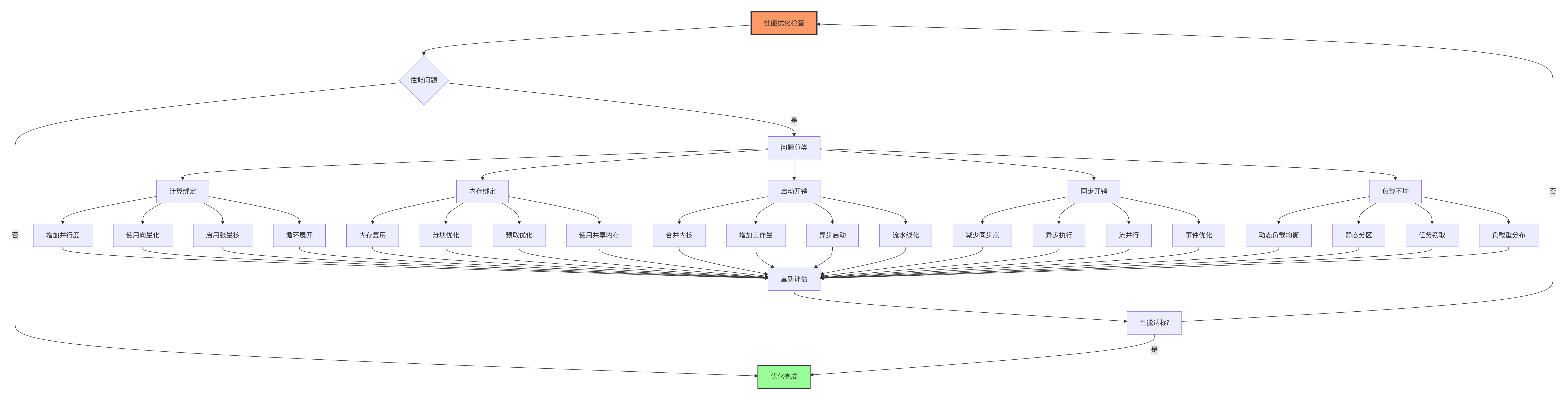
6. 性能调优检查清单
7. 总结与最佳实践
7.1 性能调优的层次
# performance_optimization_hierarchy.py
class OptimizationHierarchy:
    """优化层次结构"""

    OPTIMIZATION_LEVELS = {
        'Level 1': {
            'name': '算法级优化',
            'optimizations': [
                '选择高效算法',
                '减少计算复杂度',
                '使用近似计算',
                '提前终止计算'
            ],
            'speedup': '2-10x',
            'difficulty': '低'
        },
        'Level 2': {
            'name': '架构级优化',
            'optimizations': [
                '计算图优化',
                '算子融合',
                '内存复用',
                '流水线化'
            ],
            'speedup': '5-20x',
            'difficulty': '中'
        },
        'Level 3': {
            'name': '系统级优化',
            'optimizations': [
                '分块优化',
                '向量化',
                '预取',
                '异步执行'
            ],
            'speedup': '10-50x',
            'difficulty': '高'
        },
        'Level 4': {
            'name': '指令级优化',
            'optimizations': [
                '循环展开',
                '指令调度',
                '寄存器优化',
                '缓存优化'
            ],
            'speedup': '20-100x',
            'difficulty': '专家'
        }
    }

    def get_optimization_strategy(self, current_speedup, target_speedup):
        """获取优化策略"""
        strategies = []

        if current_speedup < 5:
            strategies.append(self.OPTIMIZATION_LEVELS['Level 1'])
        if current_speedup < 20:
            strategies.append(self.OPTIMIZATION_LEVELS['Level 2'])
        if current_speedup < 50:
            strategies.append(self.OPTIMIZATION_LEVELS['Level 3'])
        if current_speedup < 100:
            strategies.append(self.OPTIMIZATION_LEVELS['Level 4'])

        return strategies
7.2 实战经验总结
-
先分析,后优化:用数据指导优化,而不是猜测
-
分层次优化:从算法到指令逐层深入
-
小步快跑:每次优化都要验证效果
-
持续迭代:性能优化是持续过程
7.3 性能调优黄金法则
✅ 法则1:测量驱动优化 - 不测量就优化是在浪费生命
✅ 法则2:优化瓶颈 - 优化20%的关键代码解决80%的问题
✅ 法则3:分层次优化 - 从高层次到低层次,从宏观到微观
✅ 法则4:保持代码清晰 - 可读的代码比聪明但难以理解的代码更易优化
✅ 法则5:持续验证 - 每次优化都要验证正确性和性能提升
参考资料
-
Ascend C 编程指南 - 官方编程指南
-
CANN 性能优化指南 - 性能优化指南
-
NPU 架构白皮书 - 硬件架构参考
-
高性能计算优化技术 - 优化技术论文
-
数值线性代数 - 高性能计算基础
🎯 专家观点:性能优化是科学更是艺术。理解硬件、分析瓶颈、针对性优化、持续验证,这四个步骤缺一不可。真正的专家不是会调参,而是能预测性能瓶颈并系统性地解决问题。
官方介绍
昇腾训练营简介:2025年昇腾CANN训练营第二季,基于CANN开源开放全场景,推出0基础入门系列、码力全开特辑、开发者案例等专题课程,助力不同阶段开发者快速提升算子开发技能。获得Ascend C算子中级认证,即可领取精美证书,完成社区任务更有机会赢取华为手机,平板、开发板等大奖。
报名链接: https://www.hiascend.com/developer/activities/cann20252#cann-camp-2502-intro
期待在训练营的硬核世界里,与你相遇!

1331
更多推荐



 25
25 0
0- 0


 已为社区贡献7条内容

所有评论(0)